The first step in the design of a controller for a robot manipulator is to solve for its kinematics, inverse kinematics, dynamics, and the feedback control equation that will be used. Also the type of input and the user interface should be determined at this stage. We should also know the parameters of the robot, such as: link lengths, masses, inertia tensors, distances between joints, the configuration of the robot, and the type of each link (revolute or prismatic). To make a modular and flexible design, variable parameters are used that can be fed to the system at run-time, so that this controller can be used for different configurations without any changes.
Three different configurations have been chosen for development and study. The first configuration is revolute-revolute-prismatic with the prismatic link in the same plane as the first and second links. The second configuration is also revolute-revolute-prismatic with the prismatic link perpendicular to the plane of the first and second links. The last configuration is three revolute joints (see Figure 19).
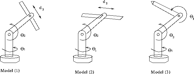
Figure 19: Three different configurations of the robot manipulator.
The kinematics and the dynamics of the three models have been
generated using some tools in the department called genkin and
gendyn that take the configuration of the manipulator in a
certain format and generate the corresponding kinematics and dynamics
for that manipulator. The kinematics and the dynamics of the three models are shown
in Appendix A. One problem with the resultant equations is that they
are not simplified at all; therefore, The results were simplified
using the mathematical package Mathematica, which gives more
simplified results, but still, not totally factorized. Appendix B
shows the dynamics after simplifying the equations using
Mathematica. The comparison between the number of calculations before
and after simplification will be discussed in the benchmarking
section.
The kinematics and the dynamics of the three models are shown
in Appendix A. One problem with the resultant equations is that they
are not simplified at all; therefore, The results were simplified
using the mathematical package Mathematica, which gives more
simplified results, but still, not totally factorized. Appendix B
shows the dynamics after simplifying the equations using
Mathematica. The comparison between the number of calculations before
and after simplification will be discussed in the benchmarking
section.
For the trajectory generation, The cubic polynomials method, described in the trajectory generation section, was used. This method is easy to implement and does not require much computation. It generates a cubic function that describes the motion from a starting point to a goal point in a certain time. Thus, this module will give us the desired trajectory to be followed, and this trajectory will serve as the input to the control module.
The error in position and velocity is calculated using the readings of the actual position and velocity from the sensors at each joint. Our control module simulated a PID controller to minimize that error. The error depends on several factors such as the frequency of update, the frequency of reading from the sensors, and the desired trajectory (for example, if we want to move through a angle in a very small time interval, the error will be large).